Tensorflow_Keras_Tutorial

Keras

• Tensorflow위에서 동작하는 라이브러리 -> 사용자 친화적으로 개발되어 사용이 편해 필요함
• 간단한 신경망의 경우 몇줄만으로 만들 수 있음
• 사용자가 Tensorflow를 좀 더 쉽고 편하게 사용할 수 있게 해주는 high level API를 제공

Tensorflow

• 구글에서 만든 딥러닝 프로그램을 쉽게 구현할 수 있도록 다양한 기능을 제공해주는 라이브러리
• TensorBoard (브라우저에서 실행가능한 시각화 도구)를 제공 -> 딥러닝 학습 과정 추적하는데 유용
• Tensor형태의 data들이 모델을 구성하는 연산들의 그래프를 따라 흐르면서 연산이 일어남 (Flow)
• Keras사용보다 훨씬 더 디테일한 조작이 가능

Tensor

• 데이터의 배열
• 배열의 집합
• array와 matrix와 매우 유사한 특수한 자료구조
• Numpy의 ndarray와 매우 유사

 

# 상수형 tensor는 아래와 같이 만들 수 있습니다
# 출력해보면 tensor의 값과 함께, shape과 내부의 data type을 함께 볼 수 있습니다
x = tf.constant([[1.0, 2.0],
                 [3.0, 4.0]])
print(x)
print(type(x))
 
# 아래와 같이 numpy ndarray나 python의 list도 tensor로 바꿀 수 있습니다
x_np = np.array([[1.0, 2.0],
                [3.0, 4.0]])
x_list = [[1.0, 2.0], 
         [3.0, 4.0]]
 
print(type(x_np))
print(type(x_list))
 
x_np = tf.convert_to_tensor(x_np)
x_list = tf.convert_to_tensor(x_list)
 
print(type(x_np))
print(type(x_list))
 
h = tf.random.uniform((2,2)) # np.rand, 균일분포
i = tf.random.normal((2,2))  # np.randn, 정규분포
print(h)
print(i)

 

Variable

변할 수 있는 상태를 저장하는데 사용되는 특별한 Tensor 

DL에서는 학습해야하는 가중치(weight, bias)들을 variable로 생성

 

# tensor의 값 변경 - 변경 불가능
tensor = tf.ones((3,4))
print(tensor)
 
tensor[0,0] = 2.
 
# variable 만들기, 값 변경
variable = tf.Variable(tensor)
print(variable)
 
variable[0,0].assign(2)
print(variable)
 
# 초기값을 사용해서 Variable을 생성할 수 있습니다
initial_value = tf.random.normal(shape=(2, 2))
weight = tf.Variable(initial_value)
print(weight)
     
# 아래와 같이 variable을 초기화해주는 initializer들을 사용할 수도 있습니다
weight = tf.Variable(tf.random_normal_initializer(stddev=1.)(shape=(2,2)))
print(weight)
 
 
# variable은 `.assign(value)`, `.assign_add(increment)`, 또는 `.assign_sub(decrement)`
# 와 같은 메소드를 사용해서 Variable의 값을 갱신합니다:'''
 
new_value = tf.random.normal(shape=(2,2))
print(new_value)
weight.assign(new_value)
print(weight)

tf.Tensor(
[[1. 1. 1. 1.]
 [1. 1. 1. 1.]
 [1. 1. 1. 1.]], shape=(3, 4), dtype=float32)

---------------------------------------------------------------------------
TypeError                                 Traceback (most recent call last)
<ipython-input-4-09e82e60b3e3> in <cell line: 5>()
      3 print(tensor)
      4 
----> 5 tensor[0,0] = 2.

TypeError: 'tensorflow.python.framework.ops.EagerTensor' object does not support item assignment

<tf.Variable 'Variable:0' shape=(3, 4) dtype=float32, numpy=
array([[1., 1., 1., 1.],
       [1., 1., 1., 1.],
       [1., 1., 1., 1.]], dtype=float32)>
<tf.Variable 'Variable:0' shape=(3, 4) dtype=float32, numpy=
array([[2., 1., 1., 1.],
       [1., 1., 1., 1.],
       [1., 1., 1., 1.]], dtype=float32)>
       
       <tf.Variable 'Variable:0' shape=(2, 2) dtype=float32, numpy=
array([[-0.47721103, -0.55552727],
       [ 0.10904223,  0.05042257]], dtype=float32)>
       
       <tf.Variable 'Variable:0' shape=(2, 2) dtype=float32, numpy=
array([[-0.2452625 , -0.8292442 ],
       [-0.21532017,  2.280255  ]], dtype=float32)>
       
       tf.Tensor(
[[0.14017352 0.41375086]
 [0.4831708  0.31189558]], shape=(2, 2), dtype=float32)
<tf.Variable 'Variable:0' shape=(2, 2) dtype=float32, numpy=
array([[0.14017352, 0.41375086],
       [0.4831708 , 0.31189558]], dtype=float32)>

 

Indexing과 Slicing

Indexing = 차원 감소, Scling = 차원 유지

 

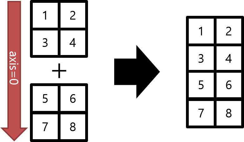
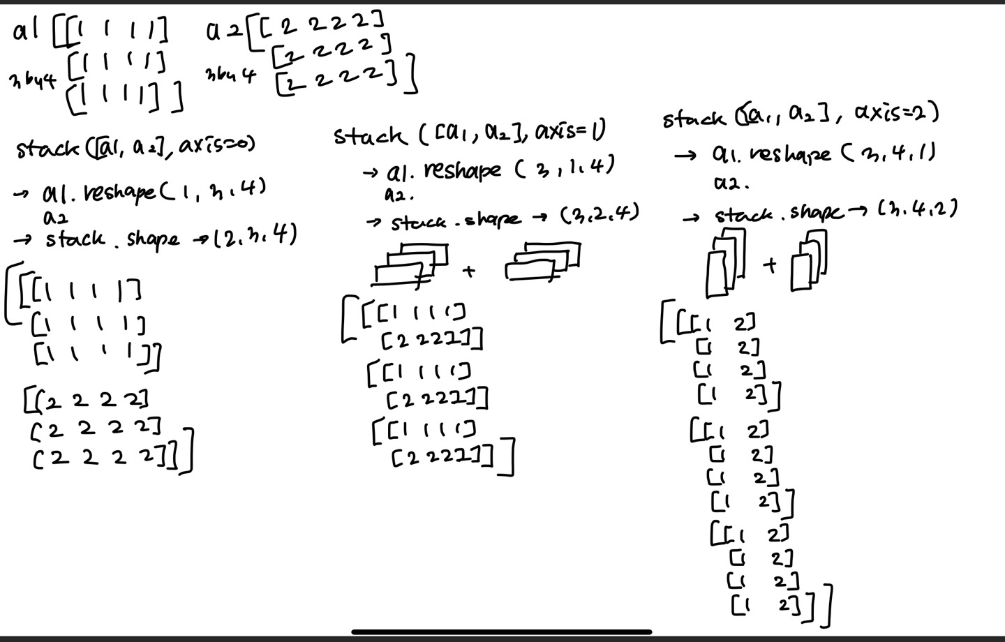
Concatenate와 Stack

concatenate - 선택한 축 방향으로 배열을 연결해주는 메소드

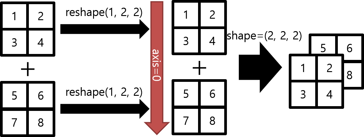
stack - 랭크 R의 tensor를 랭크 (R+1)tensor로 쌓는 메소드

 

concatenate_ex

stack_ex_axis=0

stack_ex

z = tf.range(1, 11)
z = tf.reshape(z, (2, 5))
print(z)
     
concat = tf.concat([z, z], axis=0)
print(concat)
 
concat = tf.concat([z, z], axis=-1)
print(concat)
     
# 제일 앞에 축을 생성하면서 만들어줌
stack = tf.stack([z, z], axis=0)
print(stack)
 
 
# stack은 차원을 axis방향으로 추가하고 쌓는다
# concatenate에 reshape과정(차원추가) 추가한 것 = stack
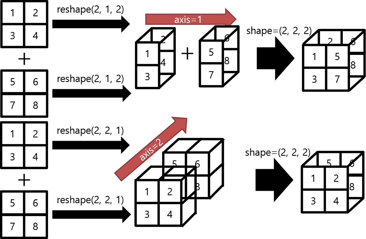
z1 = tf.reshape(z,(2,1,5))
z2 = tf.reshape(z,(1,2,5))
z3 = tf.reshape(z,(2,5,1))
 
print(z)
print(z1)
print(z2)
print(z3)
 
stack1 = tf.stack([z, z], axis=2)
stack2 = tf.stack([z,z],axis=-1)
print(stack1)
print(stack2)
     
stack = tf.stack([z, z], axis=1)
print(stack)

 

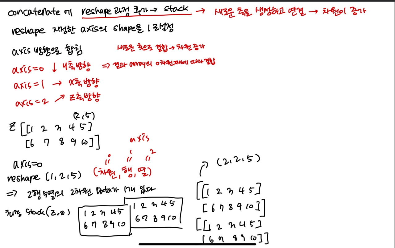
Dataset

Data를 처리하여 model에 공급하기 위하여 Tensorflow에서는 tf.data.Dataset 사용

 

FashionMNIST data 불러오기

mnist = keras.datasets.fashion_mnist
class_names = ['T-shirt/top', 'Trouser', 'Pullover', 'Dress', 'Coat', 'Sandal', 'Shirt', 'Sneaker', 'Bag', 'Ankle boot']
 
(train_images, train_labels), (test_images, test_labels) = mnist.load_data()
 
# train_images, train_labels의 shape 확인
print(train_images.shape, train_labels.shape)
 
# test_images, test_labels의 shape 확인
print(test_images.shape, test_labels.shape)
 
# training set의 각 class 별 image 수 확인
unique, counts = np.unique(train_labels, axis=-1, return_counts=True)
dict(zip(unique, counts))
 
# test set의 각 class 별 image 수 확인
unique, counts = np.unique(test_labels, axis=-1, return_counts=True)
dict(zip(unique, counts))

(60000, 28, 28) (60000,)

(10000, 28, 28) (10000,)

{0: 6000,
 1: 6000,
 2: 6000,
 3: 6000,
 4: 6000,
 5: 6000,
 6: 6000,
 7: 6000,
 8: 6000,
 9: 6000}

{0: 1000,
 1: 1000,
 2: 1000,
 3: 1000,
 4: 1000,
 5: 1000,
 6: 1000,
 7: 1000,
 8: 1000,
 9: 1000}

Data 전처리

# image를 0~1사이 값으로 만들기 위하여 255로 나누어줌
# 이미지는 255개의 픽셀로 이뤄져있다
train_images = train_images.astype(np.float32) / 255.
test_images = test_images.astype(np.float32) / 255.
 
# one-hot encoding
train_labels = keras.utils.to_categorical(train_labels, 10)
test_labels = keras.utils.to_categorical(test_labels, 10)

 

Dataset 만들기

# 학습시 이미지를 한꺼번에 한장씩이 아니라 여러장을 넣어줌 -> batch로 한번에 넣어주는 이미지 장수를 정해줌
# train_dataset은 suffle을 안해줄시, 1 epoch한 후 같은 순서로 들어감
train_dataset = tf.data.Dataset.from_tensor_slices((train_images, train_labels)).shuffle(
                buffer_size=100000).batch(64)
test_dataset = tf.data.Dataset.from_tensor_slices((test_images, test_labels)).batch(64)
 
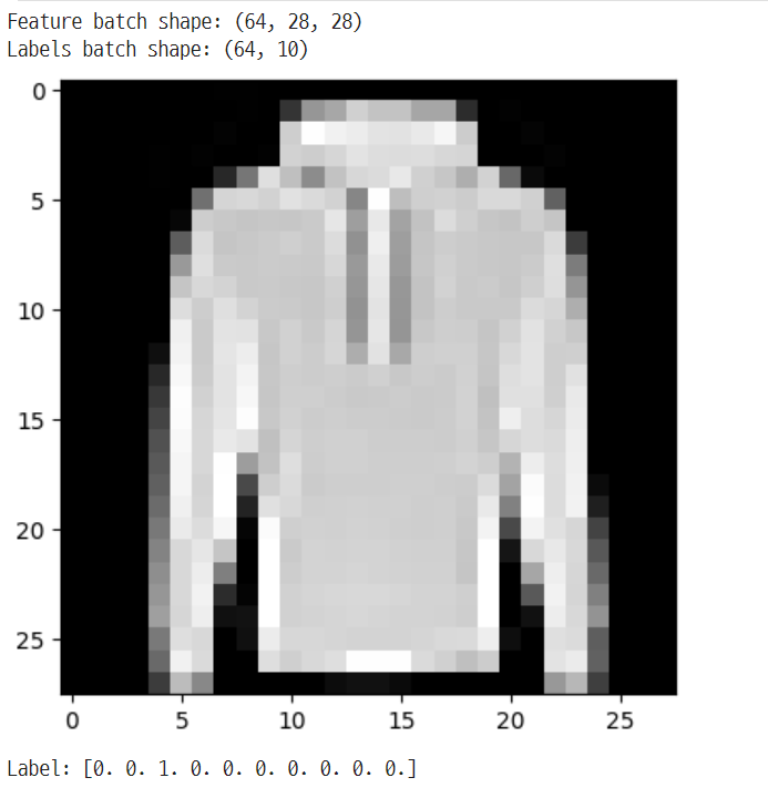
# Dataset을 통해 반복하기(iterate)
# 이미지와 정답(label)을 표시합니다.
imgs, lbs = next(iter(train_dataset))
print(f"Feature batch shape: {imgs.shape}")
print(f"Labels batch shape: {lbs.shape}")
 
img = imgs[0]
lb = lbs[0]
plt.imshow(img, cmap='gray')
plt.show()
print(f"Label: {lb}")

Custom Dataset 만들기

a = np.arange(10)
print(a)
 
ds_tensors = tf.data.Dataset.from_tensor_slices(a)
print(ds_tensors)
 
for x in ds_tensors:
    print (x)
 
# data 전처리(변환), shuffle, batch 추가
# map() -> dataset의 각 멤버에 사용자 지정 함수를 적용
# shuffle(queue의 사이즈), queue사이즈보다 data수가 많을 시 완전 shuffle
# batch(2) -> 데이터 배치의 크기, 1batch당 2개의 data
ds_tensors = ds_tensors.map(tf.square).shuffle(10).batch(2)
 
# 총 3epochs돌리는 것 
for _ in range(3):
    for x in ds_tensors:
        print(x)
    print('='*50)

[0 1 2 3 4 5 6 7 8 9]
<_TensorSliceDataset element_spec=TensorSpec(shape=(), dtype=tf.int64, name=None)>
tf.Tensor(0, shape=(), dtype=int64)
tf.Tensor(1, shape=(), dtype=int64)
tf.Tensor(2, shape=(), dtype=int64)
tf.Tensor(3, shape=(), dtype=int64)
tf.Tensor(4, shape=(), dtype=int64)
tf.Tensor(5, shape=(), dtype=int64)
tf.Tensor(6, shape=(), dtype=int64)
tf.Tensor(7, shape=(), dtype=int64)
tf.Tensor(8, shape=(), dtype=int64)
tf.Tensor(9, shape=(), dtype=int64)

tf.Tensor([ 1 81], shape=(2,), dtype=int64)
tf.Tensor([36 16], shape=(2,), dtype=int64)
tf.Tensor([ 9 49], shape=(2,), dtype=int64)
tf.Tensor([ 0 25], shape=(2,), dtype=int64)
tf.Tensor([64  4], shape=(2,), dtype=int64)
==================================================
tf.Tensor([81  4], shape=(2,), dtype=int64)
tf.Tensor([ 1 49], shape=(2,), dtype=int64)
tf.Tensor([25  0], shape=(2,), dtype=int64)
tf.Tensor([36  9], shape=(2,), dtype=int64)
tf.Tensor([16 64], shape=(2,), dtype=int64)
==================================================
tf.Tensor([25  4], shape=(2,), dtype=int64)
tf.Tensor([81 36], shape=(2,), dtype=int64)
tf.Tensor([ 0 49], shape=(2,), dtype=int64)
tf.Tensor([64  9], shape=(2,), dtype=int64)
tf.Tensor([16  1], shape=(2,), dtype=int64)
==================================================

 

 

Model

Keras에서의 모델 작성방법

1. Keras Sequential API
2. Keras Functional API
3. Model Class Subclassing

Keras Sequential API 사용

각 레이어에 정확히 하나의 입력텐서와 하나의 출력텐서가 있는 일반 레이어 스택에 적합

간단한 모델구현에 적절

단순하게 층을 쌓는 방식

 

Sequential 모델은 다음의 경우에 적합하지 않습니다.

• 다중 입력 / 다중 출력이 있는 경우
• 레이어 공유를 해야하는 경우
• 덧셈 같은 연산하는 모델 구현 시
• 비선형 토폴로지를 원할 경우

 

# multi layer perceptron
 
def create_seq_model():
  model = keras.Sequential()
  model.add(keras.layers.Flatten(input_shape=(28, 28)))
  model.add(keras.layers.Dense(128, activation='relu'))
  model.add(keras.layers.Dropout(0.2))
  model.add(keras.layers.Dense(10, activation='softmax'))
  return model
 
seq_model = create_seq_model()
 
seq_model.summary()

Model: "sequential"
_________________________________________________________________
 Layer (type)                Output Shape              Param #   
=================================================================
 flatten (Flatten)           (None, 784)               0         
                                                                 
 dense (Dense)               (None, 128)               100480    
                                                                 
 dropout (Dropout)           (None, 128)               0         
                                                                 
 dense_1 (Dense)             (None, 10)                1290      
                                                                 
=================================================================
Total params: 101,770
Trainable params: 101,770
Non-trainable params: 0
_________________________________________________________________

 

Keras Functional API 사용

Sequential보다 유연한 모델 생성

보다 복잡한 모델 생성 가능

 

def create_func_model():
  inputs = keras.Input(shape=(28,28))
  # input을 항상 명시해줘야함
  flatten = keras.layers.Flatten()(inputs)
  dense = keras.layers.Dense(128, activation='relu')(flatten)
  drop = keras.layers.Dropout(0.2)(dense)
  outputs = keras.layers.Dense(10, activation='softmax')(drop)
  model = keras.Model(inputs=inputs, outputs=outputs)
  return model
 
func_model = create_func_model()
 
func_model.summary()

Model: "model"
_________________________________________________________________
 Layer (type)                Output Shape              Param #   
=================================================================
 input_1 (InputLayer)        [(None, 28, 28)]          0         
                                                                 
 flatten_1 (Flatten)         (None, 784)               0         
                                                                 
 dense_2 (Dense)             (None, 128)               100480    
                                                                 
 dropout_1 (Dropout)         (None, 128)               0         
                                                                 
 dense_3 (Dense)             (None, 10)                1290      
                                                                 
=================================================================
Total params: 101,770
Trainable params: 101,770
Non-trainable params: 0
_________________________________________________________________

 

Model Class Subclassing 사용

Functional API가 구현할 수 없는 모델들을 구현할 수 있다.

 

class SubClassModel(keras.Model):
  def __init__(self):
    super(SubClassModel, self).__init__()
    self.flatten = keras.layers.Flatten(input_shape=(28, 28))
    self.dense1 = keras.layers.Dense(128, activation='relu')
    self.drop = keras.layers.Dropout(0.2)
    self.dense2 = keras.layers.Dense(10, activation='softmax')
  def call(self, x, training=False):
    x = self.flatten(x)
    x = self.dense1(x)
    x = self.drop(x)
    return self.dense2(x)
 
subclass_model = SubClassModel()
 
inputs = tf.zeros((1, 28, 28))
subclass_model(inputs)
subclass_model.summary()

Model: "sub_class_model"
_________________________________________________________________
 Layer (type)                Output Shape              Param #   
=================================================================
 flatten_2 (Flatten)         multiple                  0         
                                                                 
 dense_4 (Dense)             multiple                  100480    
                                                                 
 dropout_2 (Dropout)         multiple                  0         
                                                                 
 dense_5 (Dense)             multiple                  1290      
                                                                 
=================================================================
Total params: 101,770
Trainable params: 101,770
Non-trainable params: 0
_________________________________________________________________

 

Training / Validation

learning_rate = 0.001
seq_model.compile(optimizer=tf.keras.optimizers.Adam(learning_rate),
              loss='categorical_crossentropy',
              metrics=['accuracy'])
 
 
history = seq_model.fit(train_dataset, epochs=10, validation_data=test_dataset)     

Epoch 1/10
938/938 [==============================] - 6s 4ms/step - loss: 0.5576 - accuracy: 0.8042 - val_loss: 0.4379 - val_accuracy: 0.8455
Epoch 2/10
938/938 [==============================] - 3s 3ms/step - loss: 0.4112 - accuracy: 0.8522 - val_loss: 0.3932 - val_accuracy: 0.8583
Epoch 3/10
938/938 [==============================] - 3s 3ms/step - loss: 0.3721 - accuracy: 0.8641 - val_loss: 0.3805 - val_accuracy: 0.8623
Epoch 4/10
938/938 [==============================] - 3s 3ms/step - loss: 0.3489 - accuracy: 0.8723 - val_loss: 0.3708 - val_accuracy: 0.8683
Epoch 5/10
938/938 [==============================] - 4s 4ms/step - loss: 0.3372 - accuracy: 0.8772 - val_loss: 0.3534 - val_accuracy: 0.8746
Epoch 6/10
938/938 [==============================] - 3s 3ms/step - loss: 0.3214 - accuracy: 0.8807 - val_loss: 0.3534 - val_accuracy: 0.8737
Epoch 7/10
938/938 [==============================] - 3s 3ms/step - loss: 0.3120 - accuracy: 0.8849 - val_loss: 0.3460 - val_accuracy: 0.8720
Epoch 8/10
938/938 [==============================] - 4s 4ms/step - loss: 0.3014 - accuracy: 0.8890 - val_loss: 0.3470 - val_accuracy: 0.8745
Epoch 9/10
938/938 [==============================] - 3s 3ms/step - loss: 0.2925 - accuracy: 0.8918 - val_loss: 0.3434 - val_accuracy: 0.8812
Epoch 10/10
938/938 [==============================] - 3s 3ms/step - loss: 0.2842 - accuracy: 0.8939 - val_loss: 0.3576 - val_accuracy: 0.8699

 

GradientTape

Tensorflow 2.0의 자동 미분 기능 -> tf.GradientTape API 제공

컨텍스트(context) 안에서 실행된 모든 연산을 테이프(tape)에 기록

 -> 후진 방식 자동 미분(reverse mode differentiation)을 사용

 ->테이프에 "기록된" 연산의 그래디언트를 계산합니다.

1. 동적으로 Gradient 값들을 확인
2. 직접 print
3. 시각화

# loss function
loss_object = keras.losses.CategoricalCrossentropy()
 
# optimizer
learning_rate = 0.001
optimizer = keras.optimizers.Adam(learning_rate=learning_rate)
 
# loss, accuracy 계산
train_loss = keras.metrics.Mean(name='train_loss')
train_accuracy = keras.metrics.CategoricalAccuracy(name='train_accuracy')
 
test_loss = keras.metrics.Mean(name='test_loss')
test_accuracy = keras.metrics.CategoricalAccuracy(name='test_accuracy')
 
@tf.function # 데코레이터, 속도를 빠르게 해줌
def train_step(model, images, labels):
    # 미분을 위한 GradientTape을 적용
  with tf.GradientTape() as tape:
    # 1. prediction
    # training=True is only needed if there are layers with different
    # behavior during training versus inference (e.g. Dropout).
    predictions = model(images, training=True)
    # 2. loss 계산
    loss = loss_object(labels, predictions)
  # 3. gradient 계산
  gradients = tape.gradient(loss, model.trainable_variables)
  # 4. backpropagation - weight update
  optimizer.apply_gradients(zip(gradients, model.trainable_variables))
 
  # loss와 accuracy update
  train_loss(loss)
  train_accuracy(labels, predictions)

@tf.function
def test_step(model, images, labels):
  # training=False is only needed if there are layers with different
  # behavior during training versus inference (e.g. Dropout).
  predictions = model(images, training=False)
  t_loss = loss_object(labels, predictions)
 
  test_loss(t_loss)
  test_accuracy(labels, predictions)

# 실제로 학습하는 부분 
EPOCHS = 10
 
for epoch in range(EPOCHS):
  # Reset the metrics at the start of the next epoch
  train_loss.reset_states()
  train_accuracy.reset_states()
  test_loss.reset_states()
  test_accuracy.reset_states()
 
  for images, labels in train_dataset:
    train_step(func_model, images, labels)
 
  for test_images, test_labels in test_dataset:
    test_step(func_model, test_images, test_labels)
 
  print(
    f'Epoch {epoch + 1}, '
    f'Loss: {train_loss.result()}, '
    f'Accuracy: {train_accuracy.result() * 100}, '
    f'Test Loss: {test_loss.result()}, '
    f'Test Accuracy: {test_accuracy.result() * 100}'
  )

 

 

 

 

 

 

 

 

 

---

참고 및 출처 : https://backgomc.tistory.com/78 

텐서플로우 vs 케라스 간단비교

https://everyday-image-processing.tistory.com/87

넘파이 알고 쓰자 - stack, hstack, vstack, dstack, column_stack

https://teddylee777.github.io/tensorflow/gradient-tape/

[tensorflow] GradientTape의 활용법

https://www.tensorflow.org/guide/keras/save_and_serialize?hl=ko 

Keras 모델 저장 및 로드  |  TensorFlow Core