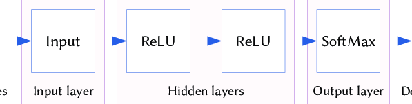
Classifier, Softmax Layer

Odds

 확률 p에 대한 odds

$O=\dfrac{p}{1-p}$

 

실패비율 대비 성공비율을 설명하는 것

Logit

확률 p의 logit

$l=\log \left( \dfrac{p}{1-p}\right) $

즉, odds에 log를 씌운 것 ( log + odds )

odds는 1보다 큰 지, logit은 0보다 큰지가 결정의 기준

logit의 역함수는 sigmoid

$l=\log \left( \dfrac{p}{1-p}\right) $

$e^{e}=\dfrac{p}{1-p}$

$\dfrac{1}{0^{1}}=\dfrac{1-p}{p}=\dfrac{1}{p}-1$

$\dfrac{1}{e^{l}}+1=\dfrac{1}{p}$

$\dfrac{e^{l}+1}{e^{l}}=\dfrac{1}{p}$

$p=\dfrac{e^{l}}{1+e^{l}}$

$p=\dfrac{1}{1+e^{-l}}=\sigma \left( l\right) $

 

→ sigmoid는 logit을 받아 확률을 계산

binary classification을 원할 때 sigmoid사용

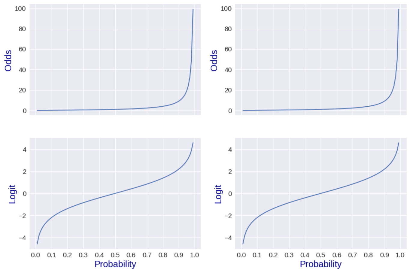
The Graphs of Odds and Logit

import numpy as np
import tensorflow as tf
 
import matplotlib.pyplot as plt
plt.style.use('seaborn')
 
# (start, stop, num(number of samples))
p_np = np.linspace(0.01, 0.99, 100)
 
p_tf = tf.linspace(0.01, 0.99, 100)
 
# odds = p / (1-p)
odds_np = p_np/(1-p_np)
odds_tf = p_tf/(1-p_tf)
 
# logit = log(p / (1-p))
logit_np = np.log(odds_np)
logit_tf = tf.math.log(odds_tf)
 
#subplots( nrows, ncolumns, figsize(단위는 inch))
fig, axes = plt.subplots(2, 2, figsize=(15, 10), sharex=True)  # x값 공유
 
# (x-axis, y-axis)
axes[0,0].plot(p_np, odds_np)
axes[1,0].plot(p_np, logit_np)
 
# (start, stop, step), x-axis
xticks = np.arange(0, 1.1, 0.1) 
axes[0,0].tick_params(labelsize=15)
axes[0,0].set_xticks(xticks)
axes[0,0].set_ylabel('Odds', fontsize=20, color='darkblue')
 
axes[1,0].tick_params(labelsize=15)
axes[1,0].set_xticks(xticks)
axes[1,0].set_ylabel('Logit', fontsize=20, color='darkblue')
axes[1,0].set_xlabel('Probability', fontsize=20, color='darkblue')
 
axes[0,1].plot(p_tf, odds_tf)
axes[1,1].plot(p_tf, logit_tf)
 
axes[0,1].tick_params(labelsize=15)
axes[0,1].set_xticks(xticks)
axes[0,1].set_ylabel('Odds', fontsize=20, color='darkblue')
 
axes[1,1].tick_params(labelsize=15)
axes[1,1].set_xticks(xticks)
axes[1,1].set_ylabel('Logit', fontsize=20, color='darkblue')
axes[1,1].set_xlabel('Probability', fontsize=20, color='darkblue')

from Logit to Probability

 

$\left( \overrightarrow{x}\right) ^{T}\rightarrow z=\left( \overrightarrow{x}\right) ^{T}\overrightarrow{w}+b\rightarrow p=\dfrac{1}{1+e^{-z}}$

 

$-\infty \leq z <\infty $, $0\leq p\leq 1$

==> sigmoid function과 동일

 

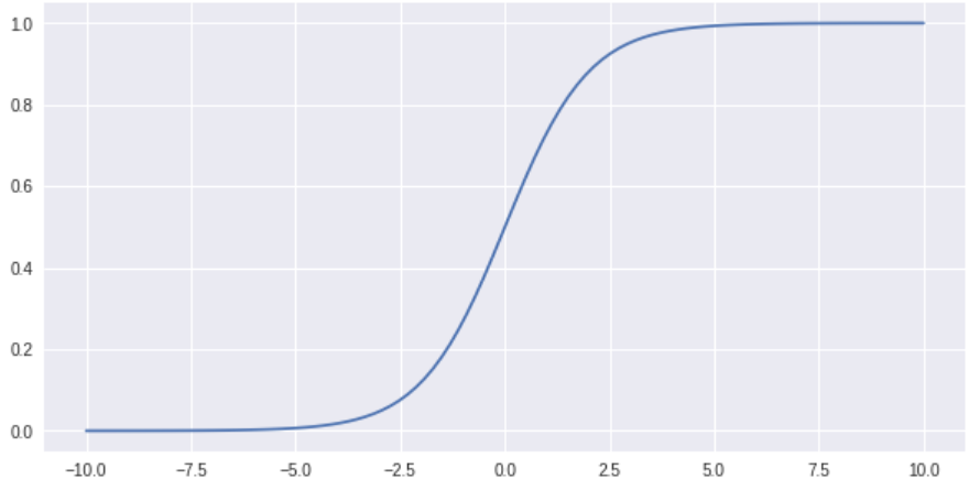
The Graphs of Sigmoid

import tensorflow as tf
 
from tensorflow.keras.layers import Activation
 
# (start, stop, num(number of samples))
x = tf.linspace(-10, 10, 100)
sigmoid = Activation('sigmoid')(x)
 
fig, ax = plt.subplots(figsize=(10, 5))
ax.plot(x.numpy(), sigmoid.numpy())

 

Logistic Regression

실제로 많은 특정변수에 대한 확률값이 선형이 아닌 S-curve형태인 경우가 많음

S-curve를 함수로 표현해낸 것 = Logistic Function (Sigmoid Function이라 부르기도 함)

→ x값으로 어떤 값이든 받을 수 있으나 output은 항상 0~1 사이값

 

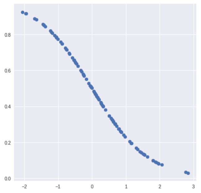
Single_variate Logistic Regression Models

import matplotlib.pyplot as plt
import tensorflow as tf
from tensorflow.keras.layers import Dense
 
plt.style.use('seaborn')
 
# 100 by 1 matrix, feature 1개
x = tf.random.normal(shape=(100, 1))
dense = Dense(units=1, activation='sigmoid')
 
Y = dense(x)
 
fig, ax = plt.subplots(figsize=(7, 7))
print(Y.shape)
ax.scatter(x.numpy().flatten(), Y.numpy().flatten())

results
(100, 1)

 

Multi_variate Logistic Regression Models

import matplotlib.pyplot as plt
import tensorflow as tf
from tensorflow.keras.layers import Dense
 
plt.style.use('seaborn')
 
# feature가 5개, 100 by 5 matrix
x = tf.random.normal(shape=(100, 5))   
dense = Dense(units=1, activation='sigmoid')
 
Y = dense(x)
print(Y.shape)

Softmax Layer

 

logit vector를 받아 probability vector로 바꿔주는 레이어

입력받은 값을 출력으로 0~1 사이의 값으로 모두 정규화하여 출력값들의 총합은 1이 되는  특성

→ 확률이기 때문 ($0\leq p\leq 1$)

주로 multi-class calssification에서 사용, 출력단에 사용

softmax function의 특징
1. 출력은 항상 0~1 사이의 실수
2. 출력의 총합은 항상 1
→2에 의해 확률로 해석할 수 있다, 확률의 범위 = 
($0\leq p\leq 1$)

softmax function
$S_{j}\left( \left( \overrightarrow{l}\right) ^{T}\right) =p_{j}=\dfrac{e^{lj}}{\sum ^{K}_{k=1}\left[ e^{l_k}\right] }$

$p_{i}=P\left( C_{i}\right) ,1\leq i <K$ ,  C = class, p = probability

동작 순서

1. 여러 개의 logit vector $\left( \overrightarrow{l}\right) ^{T}$ 가 softmax layer의 input으로 들어감
2. $l_{1}$ ($C_{1}$에 대한 logit)을 softmax에 통과
3. $p_{1}$ 으로 바뀌어 나옴

import tensorflow as tf
 
from tensorflow.keras.layers import Activation
 
logit = tf.random.uniform(shape=(8, 5), minval = -10, maxval = 10)
softmax_value = Activation('softmax')(logit)
# axis = 1 -> 열
softmax_sum = tf.reduce_sum(softmax_value, axis=1) 
 
print("Logits: \n",logit.numpy())
print("Probabilities : \n", softmax_value.numpy())
print("Sum of softmax values: \n", softmax_sum)  # sum = 1이여야함

results
Logits: [[-1.916687 -5.733509 3.7484627 -7.279396 -4.2998385 ]
[-9.271793 8.50437 1.3734322 8.120691 2.5568504 ]
[-6.518402 -8.907463 -1.1298084 -9.354267 -3.547089 ]
[-5.0065923 1.9698887 -2.3188806 8.167702 3.2706976 ]
[ 2.5599842 0.04105759 -5.241158 -0.03053665 -1.3174458 ]
[-3.8684416 6.427862 -5.7993507 -8.006101 4.8766327 ]
[ 1.5249968 -1.7952442 0.8241539 -0.648551 1.1239719 ]
[ 1.5017242 3.2117252 3.6775284 -4.457059 -6.321852 ]]
Probabilities : [[3.4512498e-03 7.5919204e-05 9.9613827e-01 1.6180109e-05 3.1840993e-04]
[1.1307632e-08 5.9355533e-01 4.7482588e-04 4.0441921e-01 1.5505522e-03]
[4.1742632e-03 3.8284578e-04 9.1372675e-01 2.4489468e-04 8.1471302e-02]
[1.8808609e-06 2.0146689e-03 2.7644903e-05 9.9055743e-01 7.3984000e-03]
[8.4987754e-01 6.8454251e-02 3.4782704e-04 6.3724644e-02 1.7595837e-02]
[2.7852233e-05 8.2506454e-01 4.0390278e-06 4.4452636e-07 1.7490311e-01]
[4.3183157e-01 1.5608173e-02 2.1426055e-01 4.9130887e-02 2.8916886e-01]
[6.5183885e-02 3.6039951e-01 5.7422215e-01 1.6837344e-04 2.6085811e-05]]
Sum of softmax values:
tf.Tensor( [1. 0.9999999 1.0000001 1. 1.0000001 0.99999994 1. 1. ], shape=(8,), dtype=float32)

Softmax in Dense layer

from os import access
import tensorflow as tf
 
from tensorflow.keras.layers import Dense
 
# 균등분포, 8 by 5 matrix
logit = tf.random.uniform(shape=(8, 5), minval = -10, maxval = 10)
# unit은 neuron의 갯수
dense = Dense(units=8, activation='softmax')
 
Y = dense(logit)
print(tf.reduce_sum(Y, axis=1))

Binary Classification 

이항분류

2개의 label을 갖는 data가 들어왔을때, 0 / 1로 분류하는 것
규칙에 따라 입력된 값을 두 그룹으로 분류 - 결과가 T / F나 A,B그룹으로 나누는 경우
주로 sigmoid를 사용하나, softmax도 사용가능

import tensorflow as tf
from tensorflow.keras.layers import Dense
from tensorflow.keras.models import Sequential
 
# Sequential modle은 하나의 입력과 하나의 출력이 있어야함
model = Sequential()
model.add(Dense(units=10, activation='relu'))
model.add(Dense(units=5, activation='relu'))
model.add(Dense(units=1, activation='sigmoid'))  # binary classifier가 될 수 있음

 

Sequential model
각 레이어에 정확히 하나의입력 텐서와 하나의 출력 텐서가 있는 일반 레이어 스택에 적합

단순히 이전 layer의 output이 다음 layer의 input으로 들어가는 선형적인 경우 편리

-> 단점 : DenseNet()같이 선형적 흐름이 아닌 모델 설계엔 사용불가

# Define Sequential model with 3 layers
model = keras.Sequential(
    [
        layers.Dense(2, activation="relu", name="layer1"),
        layers.Dense(3, activation="relu", name="layer2"),
        layers.Dense(4, name="layer3"),
    ]
)
# Call model on a test input
x = tf.ones((3, 3))
y = model(x)
 
# 위, 아래 결과 동일
 
# Create 3 layers
layer1 = layers.Dense(2, activation="relu", name="layer1")
layer2 = layers.Dense(3, activation="relu", name="layer2")
layer3 = layers.Dense(4, name="layer3")
 
# Call layers on a test input
x = tf.ones((3, 3))
y = layer3(layer2(layer1(x)))

Multi-class Classification

다중분류input을 3그룹 이상으로 분류하는 작업
하나의 feature나 여러 feature에서 나온 값을 계산 → 각 class에 속할 확률 계산

→ multi class classification에서 마지막 layer neuron갯수 = 구분하고 싶은 class 의 갯수로 설정

tf.keras.Model()

인풋텐서와 아웃풋 첸서가 주어졌을 떄, 모델을 다음과 같이 인스턴스화 할 수 있다

모델은 a를 받아 b를 계산하는데 필요한 모든 레이어 포함

다중 인풋 혹은 다중 아웃풋 모델의 경우 리스트 사용할 수 있다

Sequential()의 불편한 점 해결가능 → Multi Input / Multi Output 지원

 

Multi-class Classifiers

import tensorflow as tf
 
from tensorflow.keras.models import Model
from tensorflow.keras.layers import Dense
 
class TestModel(Model):
  def __init__(self):
    super(TestModel, self).__init__()
 
    self.dense1 = Dense(units=8, activation='relu')
    self.dense2 = Dense(units=5, activation='relu')
    self.dense3 = Dense(units=3, activation='softmax')
 
  def call(self, x):
    print("X : {}\n{}\n".format(x.shape, x.numpy()))
 
    x = self.dense1(x)
    print("A1: {}\n{}\n".format(x.shape, x.numpy()))
    
    x = self.dense2(x)
    print("A2: {}\n{}\n".format(x.shape, x.numpy()))
    
    x = self.dense3(x)
    print("Y: {}\n{}\n".format(x.shape, x.numpy()))
    print("Sum of vectors: {}\n".format(tf.reduce_sum(x, axis=1)))
    return x
 
model = TestModel()
 
X = tf.random.uniform(shape=(8, 5), minval = -10, maxval = 10)
Y = model(X)

results
X : (8, 5)
[[ 2.7306414 -4.5043635 9.202312 -9.729929 4.5601654 ]
[-9.43515 -3.2731962 2.7073717 -1.8210602 6.039503 ]
[-2.608459 9.926994 -3.7898111 -9.658632 8.525955 ]
[-8.141861 7.6586723 -1.4186335 -7.7409053 7.511627 ]
[ 7.6202927 -7.5814915 9.817312 -1.3243027 -8.664522 ]
[ 5.2555637 -4.334736 -2.3588896 0.70489883 2.0085258 ]
[ 4.0495033 -4.555273 7.438957 8.257582 -3.7457752 ]
[ 1.2603779 -6.1622357 -9.3884735 7.5500984 3.566759 ]]
A1: (8, 8)
[[ 0. 0. 4.223045 0. 0. 2.1976156 0. 0. ]
[ 4.4849157 0. 0. 3.895809 0. 6.2977552 3.4857292 0. ]
[ 3.232225 0. 0. 0. 0. 0. 6.2667346 0. ]
[ 6.5099583 0. 0. 3.0640934 0. 0.24818487 8.033037 0. ]
[ 0. 0. 11.908857 0. 0.83686936 0.45559946 0. 5.3130994 ]
[ 0. 5.422878 1.9798303 0. 0. 0. 0. 1.1099018 ]
[ 0. 0.18014723 7.4350653 0.87399757 5.889718 1.4400728 0. 5.6244946 ]
[ 0. 9.480818 0. 0.8532674 0. 1.7257781 0. 0.27880406]]
A2: (8, 5)
[[0.6331496 1.002812 0.88288766 1.0736346 0. ]
[0. 3.8800874 2.0037718 2.707113 0. ]
[0. 0.67626435 0. 0.8038477 4.263638 ]
[0. 3.3368769 0. 4.0273914 4.902274 ]
[0. 3.1042101 2.0191374 3.3771036 0. ]
[0. 0. 1.7897258 3.6184292 0. ]
[0. 4.0904217 2.7249293 0. 0. ]
[0. 0. 2.8164947 5.191123 0. ]]
Y: (8, 3)
[[0.5043968 0.32740808 0.16819513]
[0.85681885 0.09126266 0.05191846]
[0.9698344 0.02114226 0.00902322]
[0.984922 0.01275515 0.0023229 ]
[0.8029191 0.16710743 0.02997344]
[0.42978847 0.56092685 0.00928471]
[0.9140235 0.01608065 0.06989583]
[0.44923264 0.5494427 0.00132473]]
Sum of vectors: [1. 0.99999994 0.9999998 1. 0.99999994 1. 1. 1.0000001 ]

Sigmoid와 Softmax차이

입력받는 logit의 갯수 차이
sigmoid는 logit 1개를 , softmax는 logit vector를 입력받음

softmax는 여러개의 입력을 받아 여러개의 출력을 나오게 함

sigmoid통과시
마지막 layer에 neuron 1개를 깔고 sigmoid통과시킴 → $p( c= 1) $ 이 나옴 →$p(c= 0) =1-p(c=1) $ 으로 구함
softmax통과시
마지막 layer에 neuron 2개를 깔고 softmax통과시킴 → $p(c_1), p(c_2) $가 나옴

 

---

참고 및 출처 : https://www.researchgate.net/figure/Neural-network-structure-of-MLID-Input-dense-layer-two-hidden-dense-layers-with-ReLU_fig3_341062291 , https://haje01.github.io/2019/11/19/logit.html , https://m.blog.naver.com/wideeyed/221021710286 , https://velog.io/@developerkerry/Softmax-%ED%99%9C%EC%84%B1%ED%99%94-%ED%95%A8%EC%88%98 , https://androidkt.com/implement-softmax-and-cross-entropy-in-python-and-pytorch/ , https://www.tensorflow.org/guide/keras/sequential_model?hl=ko ,