Artificial Neuron

Tensor

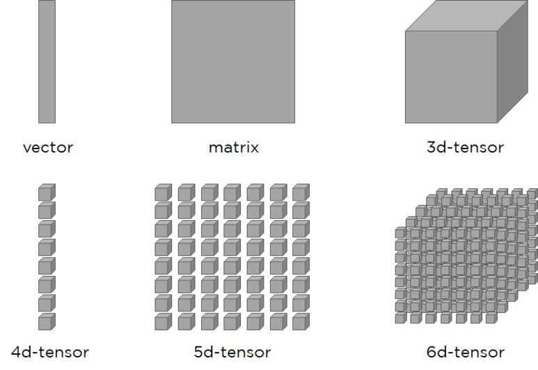
Zeroth- order Tensor ( 0차원 텐서 ) = scalar
First-order Tensor(1차원 텐서) = vector
Second-order Tensor( 2차원 텐서) = matrix

※ 위와 같이 나눌 수 있으나, 모두 Tensor로 표현 가능

 

데이터의 배열, 다차원의 배열을 통칭

scalar, vector, matrix를 general하게 표현한 것

Dataset

$\overrightarrow{X}^{T}=\left( x_{1}x_{2}\ldots x_{l_{I}}\right) $

 

주로 column형식의 벡터로 표현

 

$X^{T}=\begin{pmatrix}
X^{\left( 1\right) } \\
\chi ^{\left( 2\right) } \\
: \\
X^{(N)}
\end{pmatrix}$

 

$X^{T}=\begin{pmatrix}
\leftarrow \left( \overrightarrow{x}^{\left( 1\right) }\right) ^{T}\rightarrow  \\
\leftarrow \left( \overrightarrow{x}^{\left( 2\right) }\right) ^{T}\rightarrow  \\
: \\
t\left( \overrightarrow{x}^{\left( n\right) }\right) ^{T}-
\end{pmatrix}$

 

Weight

가중치
각 입력신호에 부여되어 입력신호와의 계산, 신호의 총합이 정해진 임계값을 넘었을 때 1 출력 
각 입력신호에는 고유한 가중치가 부여
클수록 해당 신호가 중요
기계학습이 하는 일은 이 가중치의 값을 정하는 작업
입력신호가 결과출력에 주는 영향도를 조절하는 매개변수

Bias

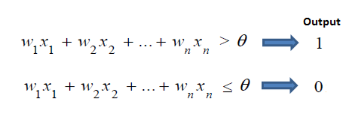
편향 (b, 그림에선 θ)
input이 가중치와 계산되어 넘어야하는 임계점
값이 높을수록 분류기준이 엄격
바이어스가 높을 수록 모델이 간단 → 과적합(overfitting)의 위험이 발생
바이어스가 낮을수록 한계점이 낮음 → 데어터의 허용범위가 넓어짐
→ 모델 복잡,필요없는 노이즈 포함가능성↑
뉴런이 얼마나 쉽게 활성화되느냐를 조정하는 매개변수

값이 높을수록 분류기준이 엄격
바이어스가 높을 수록  →  모델이 간단 → 과적합(overfitting)의 위험이 발생
바이어스가 낮을수록  →  한계점이 낮음 → 데이터의 허용범위가 넓어짐 → 모델 복잡, 필요없는 노이즈 포함가능성↑

Affine Function

Affine Transformation을 수행하기 위한 함수

 

$ z = xw+b $ 

Affine Transformation ( 어파인 변환)
신경망 forward propagation에서 수행하는 행렬의 곱을 기하학에서 부르는 이름
선형변환 중 하나로, 점, 직선, 평면을 보존한다.

 

import tensorflow as tf
 
from tensorflow.keras.layers import Dense # keras에서 dense layer 만듬 
 
x = tf.constant([[10.]])  # input setting (Note: input -> matrix)
 
#imp. an affine function, w,b  여기서 initialization이 되지않음
#unit 1개를 이용해 affine function을 만들 수 있다
#activation='linear'로 하면 z값자체가 output으로 만들어짐
dense = Dense(units=1, activation='linear')
 
# forward propagation + params initialization ,z연산
# x값이 통과할때 초기화를 시킴, x 갯수에 따라 w와 b를 초기화시켜주도록 작동, 통과해야 w,b가 만들어짐
y_tf = dense(x)
# get weight, bias
W, B = dense.get_weights()
 
#forward propagation(manual) 직접 계산
y_man = tf.linalg.matmul(x, W) + B   
 
#print results
print('==== Input/Weight/Bias====')
print("x: {}\n{}\n".format(x.shape, x.numpy()))
print("W: {}\n{}\n".format(W.shape, W))
print("B: {}\n{}\n".format(B.shape, B))
 
print('====Output====')
print("y(Tensorflow): {}\n{}\n".format(y_tf.shape, y_tf.numpy())) 
print("y(Manual): {}\n{}\n".format(y_man.shape, y_man.numpy()))

results - 

==== Input/Weight/Bias====
x: (1, 1)
[[10.]]
W: (1, 1)
[[1.634482]]
B: (1,)
[0.]
====Output====
y(Tensorflow): (1, 1)
[[16.34482]]
y(Manual): (1, 1)
[[16.34482]]

Affine Functions with 1 feature

weight sum 
$z=xw$
Affine Transformation
$ z = xw+b $ 

 

import tensorflow as tf
 
from tensorflow.keras.layers import Dense
from tensorflow.keras.initializers import Constant
 
# input setting
x = tf.constant([[10.]]) 
 
#weight/bias setting
#tensorflow는 floating point 32bit로 움직임, 숫자 뒤 점 습관화하기 
w, b = tf.constant(10.), tf.constant(20.) 
 
#tf.keras.initializers.Constant() = Constant()
# 텐서값이 아니라 w,b를 초기화시켜주는 오브젝트가 나옴, 단순히 텐서값 포함이 아니다
w_init, b_init = Constant(w), Constant(b)  
 
 
# imp. an affine function 
dense = Dense(units=1, activation='linear', kernel_initializer=w_init,bias_initializer=b_init)
 
y_tf = dense(x)
print(y_tf)  # 10*10+20 = 120 (x*w+b)
W, B = dense.get_weights()
 
#print results
print("W : {}\n{}\n".format(W.shape, W))
print("B : {}\n{}\n".format(B.shape, B))
 
# 회귀, 로지스틱 회귀에 사용

tf.Tensor([[120.]], shape=(1, 1), dtype=float32)
W : (1, 1)
[[10.]]
B : (1,)
[20.]

 

Affine Functions with n features

weight sum 
$z=w_{1}x_{1}+w_{2}x_{2}+\ldots +w_{n}x_{n}=\left( \overrightarrow{x}\right) ^{T}\overrightarrow{w}$
Affine Transformation
$z=w_{1}x_{1}+w_{2}x_{2}+\ldots +w_{n}x_{n}+b=\left( \overrightarrow{x}\right) ^{T}\overrightarrow{w}+b$

 

import tensorflow as tf
 
from tensorflow.keras.layers import Dense
 
# 랜덤모듈에서 1~10 사이 골고루 나오도록, x vector가 (1,10)행렬
x = tf.random.uniform(shape=(1,10)) 
 
# weight가 몇개 들어가야하는지 모르는 상황
dense = Dense(units=1) 
 
#통과하면 weight가 몇개 들어가야하는지 설정이 됨, weight10개, bias1개 초기화시켜줘야함
y_tf = dense(x)  
 
W, B = dense.get_weights()  
 
y_man = tf.linalg.matmul(x, W) + B  
 
#print results
print('==== Input/Weight/Bias====')
print("x: {}\n{}\n".format(x.shape, x.numpy()))
print("W: {}\n{}\n".format(W.shape, W))  # column vector로 출력, weight vector (w1~w10)
print("B: {}\n{}\n".format(B.shape, B))  # bias는 1개
 
print('====Output====')
print("y(Tensorflow): {}\n{}\n".format(y_tf.shape, y_tf.numpy())) 
print("y(Manual): {}\n{}\n".format(y_man.shape, y_man.numpy()))

results - tensorflow값과 manual값이 일치 

==== Input/Weight/Bias====
x: (1, 10)
[[0.9617789 0.13603842 0.18825376 0.69937634 0.67656493 0.67599976 0.24775136 0.833496 0.49840224 0.41456854]]
W: (10, 1)
[[-0.05368286] [ 0.60565907] [-0.600706 ] [-0.10590523] [ 0.05996251] [ 0.15246284] [ 0.21105611] [ 0.10811931] [-0.6835115 ] [-0.17381865]]
B: (1,)
[0.]
====Output====
y(Tensorflow): (1, 1)
[[-0.2830745]]
y(Manual): (1, 1)
[[-0.2830745]]

Actvation Function

활성화 함수
입력된 데이터의 가중 합을 출력신호로 변환하는 함수
입력 신호의 총합을 출력신호로 변환하는 함수

 

모델의 복잡도를 올리기 위해 필요

이전 층의 결과값을 변환하여 다른 층의 뉴런으로 신호를 전달하는 역할

 

인공신경망에서 이전 레이어에 대한 가중 합의 크기에 따라 활성여부가 결정

신경망의 목적에 따라, 혹은 레이어의 역할에 따라 선택적으로 적용

입력받은 신호를 얼마나 출력할지 결정하고 네트워크에 층을 쌓아 비선형성을 표현 할 수 있도록 해줌

 

활성화 함수가 비선형 함수여야 하는 이유 
 선형함수는 출력이 입력의 상수 배 만큼 변화하는 함수로, 
 선형함수를 사용할 시 신경망의 층을 깊게하는 의미가 없다
 층을 아무리 깊게 해도 은닉층이 없는 네트워크로, 여러층으로 구성하기 힘듬

 

활성화 함수의 종류

1.  Sigmoid   $\sigma \left( x\right) =\dfrac{1}{1+e^{-x}}$
2.  Tanh   $\tanh \left( x\right) =\dfrac{e^{x}-e^{-x}}{e^{x}+e^{-x}}$
3.  ReLU   $ReLU\left( x\right) =\max \left( 0,x\right) $  (x값이 0보다 작을 때 0 출력)

Activation function 구현

# activation fucn만 만드는 법
 
import tensorflow as tf
from tensorflow.math import exp, maximum
from tensorflow.keras.layers import Activation
 
#input setting 
x = tf.random.normal(shape=(1,5))
 
# imp. activation function
 
sigmoid = Activation('sigmoid')
tanh = Activation('tanh')
relu = Activation('relu')
 
# forward propagation(Tensorflow)
y_sigmoid_tf = sigmoid(x)
y_tanh_tf = tanh(x)
y_relu_tf = relu(x)
 
# forward propagation(manual)
 
y_sigmoid_man  = 1 / (1 + exp(-x))
y_tanh_man = (exp(x) - exp(-x)) / (exp(x) + exp(-x))
y_relu_man = maximum(0,x)
 
print("x : {}\n{}".format(x.shape, x.numpy()))
print("Sigmoid(Tensorflow): {}\n{}".format(y_sigmoid_tf.shape, y_sigmoid_tf.numpy()))
print("Sigmoid(manual): {}\n{}".format(y_sigmoid_man.shape, y_sigmoid_man.numpy()))
 
print("Tanh(Tensorflow): {}\n{}".format(y_tanh_tf.shape, y_tanh_tf.numpy()))
print("Tanh(manual): {}\n{}".format(y_tanh_man.shape, y_tanh_man.numpy()))
 
print("ReLU(Tensorflow): {}\n{}".format(y_relu_tf.shape, y_relu_tf.numpy()))
print("ReLU(manual): {}\n{}".format(y_relu_man.shape, y_relu_man.numpy()))

results - tensorflow값과 manual값이 일치 

x : (1, 5)
[[ 1.807891 1.2539947 -0.93710077 -0.13290061 -0.48402297]]
Sigmoid(Tensorflow): (1, 5)
[[0.8591068 0.7779906 0.28148636 0.46682367 0.3813026 ]]
Sigmoid(manual): (1, 5)
[[0.8591068 0.7779906 0.28148636 0.46682364 0.38130262]]
Tanh(Tensorflow): (1, 5)
[[ 0.9476171 0.84940004 -0.7338874 -0.13212363 -0.4494597 ]]
Tanh(manual): (1, 5)
[[ 0.9476172 0.84940004 -0.7338874 -0.13212363 -0.4494597 ]]
ReLU(Tensorflow): (1, 5)
[[1.807891 1.2539947 0. 0. 0. ]]
ReLU(manual): (1, 5)
[[1.807891 1.2539947 0. 0. 0. ]]

Activation function in Dense layer 구현

# Dense Layer안에 activation function 구현하기
 
import tensorflow as tf
from tensorflow.math import exp, maximum
from tensorflow.keras.layers import Dense
 
x = tf.random.normal(shape=(1,5))  #input setting 
 
# imp. artificial neurons
dense_sigmoid = Dense(units=1, activation='sigmoid')  # affine + activation
dense_tanh = Dense(units=1, activation='tanh')
dense_relu = Dense(units=1, activation='relu')
 
# forward propagation(Tensorflow)
y_sigmoid = dense_sigmoid(x)
y_tanh = dense_tanh(x)
y_relu = dense_relu(x)
 
# print resluts
print("AN with Sigmoid: {}\n{}".format(y_sigmoid.shape, y_sigmoid.numpy()))
print("AN with Tanh: {}\n{}".format(y_tanh.shape, y_tanh.numpy()))
print("AN with ReLU: {}\n{}".format(y_relu.shape, y_relu.numpy()))
 
# forward propagation(manual)
print('\n====\n')
 
W_sigmoid, B_sigmoid = dense_sigmoid.get_weights()
z = tf.linalg.matmul(x,W_sigmoid) + B_sigmoid
a_sigmoid  = 1 / (1 + exp(-z))
print("Activation Sigmoid value(Tensorflow): {}\n{}".format(y_sigmoid.shape, y_sigmoid.numpy()))
print("Activation Sigmoid value(manual): {}\n{}".format(a_sigmoid.shape, a_sigmoid.numpy()))
 
W_tanh, B_tanh = dense_tanh.get_weights()
z_tanh = tf.linalg.matmul(x,W_tanh) + B_tanh
a_tanh  = (exp(z_tanh) - exp(-z_tanh)) / (exp(z_tanh) + exp(-z_tanh))
print("Activation Tanh value(Tensorflow): {}\n{}".format(y_tanh.shape, y_tanh.numpy()))
print("Activation Tanh value(manual): {}\n{}".format(a_tanh.shape, a_tanh.numpy()))
 
W_relu, B_relu = dense_relu.get_weights()
z_relu = tf.linalg.matmul(x,W_relu) + B_relu
a_relu  = maximum(0,z_relu)
print("Activation ReLU value(Tensorflow): {}\n{}".format(y_relu.shape, y_relu.numpy()))
print("Activation ReLU value(manual): {}\n{}".format(a_relu.shape, a_relu.numpy()))

results - tensorflow값과 manual값이 일치 

AN with Sigmoid: (1, 1)
[[0.48862118]]
AN with Tanh: (1, 1)
[[-0.06860781]]
AN with ReLU: (1, 1)
[[0.]]
====
Activation Sigmoid value(Tensorflow): (1, 1)
[[0.48862118]]
Activation Sigmoid value(manual): (1, 1)
[[0.48862115]]
Activation Tanh value(Tensorflow): (1, 1)
[[-0.06860781]]
Activation Tanh value(manual): (1, 1)
[[-0.0686078]]
Activation ReLU value(Tensorflow): (1, 1)
[[0.]]
Activation ReLU value(manual): (1, 1)
[[0.]]

Artificial Neurons

$\left( \overrightarrow{x}\right) ^{T}\rightarrow f\left( \left( \overrightarrow{x}\right) ^{T};\overrightarrow{w},b\right) \dfrac{z\in \mathbb{R} }{},g\left( z\right) \dfrac{a\in \mathbb{R} }{}a$

 

import tensorflow as tf
from tensorflow.keras.layers import Dense
from tensorflow.math import exp, maximum
 
#activation = 'sigmoid'
#activation = 'tanh'
activation = 'relu'
 
#input setting
x = tf.random.uniform(shape=(1,10))
 
#imp. an affine + activation
dense = Dense(units=1, activation=activation) 
y_tf = dense(x)
W, B = dense.get_weights()
 
#calculate activation value manually
y_man = tf.linalg.matmul(x,W) + B
if activation == 'sigmoid' :
  y_man = 1 / (1 + exp(-y_man))
elif activation == 'tanh' :
  y_man = (exp(y_man) - exp(-y_man)) / (exp(y_man) + exp(-y_man))
elif activation == 'relu' :
  y_man = maximum(0,y_man)
 
print("Activation: ", activation)
print("y_tf: {}\n{}\n".format(y_tf.shape, y_tf.numpy()))
print("y_man: {}\n{}\n".format(y_man.shape, y_man.numpy()))

results - tensorflow값과 manual값이 일치 

Activation: relu
y_tf: (1, 1)
[[0.48963225]]
y_man: (1, 1)
[[0.48963225]]

Input이 Minibatch일 경우 구현

shapes in Dense layers

import tensorflow as tf
from tensorflow.keras.layers import Dense
 
# set input params
N, n_feature = 8, 10
# generate minibatch
x = tf.random.normal(shape=(N, n_feature))  # matrix형태, 8행10열
 
# imp. an AN
dense = Dense(units=1,activation='relu')
#forward propagation
y = dense(x)
 
# get weight/bias
W, B = dense.get_weights()
 
#print results
print("Shape of x: {}", x.shape)
print("Shape of W: {}", W.shape)
print("Shape of B: {}", B.shape)

results

Shape of x: {} (8, 10)
Shape of W: {} (10, 1)
Shape of B: {} (1,)

Output calculation

import tensorflow as tf
from tensorflow.keras.layers import Dense
 
# set input params
N, n_feature = 8, 10
# generate minibatch
x = tf.random.normal(shape=(N, n_feature))  # matrix형태, 8행10열
 
# imp. an AN
dense = Dense(units=1,activation='sigmoid')
#forward propagation(Tensorflow)
y_tf = dense(x)
 
W, B = dense.get_weights()
 
#forward propagation(Tensorflow)
y_man = tf.linalg.matmul(x,W) + B
y_man = 1 / (1 + tf.math.exp(-y_man))
# print results
print("Output(Tensorflow): \n", y_tf.numpy())
print("Output(manual): \n", y_man.numpy())
#print(tf.math.equal(y_tf, y_man))  # floating point가 잘려 나와 항상 True가 아니다

results - tensorflow값과 manual값이 일치 

Output(Tensorflow):
[[0.48920912]
[0.57421196]
[0.47956005]
[0.5983009 ]
[0.5136241 ]
[0.35580188]
[0.7624293 ]
[0.80499876]]
Output(manual):
[[0.48920915]
[0.574212 ]
[0.47956005]
[0.5983009 ]
[0.5136241 ]
[0.35580185]
[0.76242924]
[0.80499876]]

---

참고 : https://rekt77.tistory.com/102 , https://syj9700.tistory.com/37, https://happy-obok.tistory.com/55  , https://sacko.tistory.com/10 ,